Methods for Determining Boundary Conditions for Rod Models
Published:
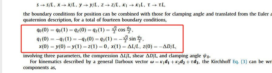
How to determine the boundary conditions of a rod?
Euler angle rotations in three-dimensional space can be difficult to fully comprehend at once when they are complex. How can we determine the correct boundary conditions for a Kirchhoff rod? A direct solution method is presented below.
Expressing the rod ends in global and local frames
Assume the global frame is represented by the identity matrix $\mathbf{E}$, the left-end local frame is $\mathbf{D_0}$, and the right-end local frame is $\mathbf{D_1}$. The global and local frames are related through rotation matrices:
\[\mathbf{D}_0=\mathbf{R}_0\mathbf{E}\] \[\mathbf{D}_1=\mathbf{R}_1\mathbf{E}\]We only need to solve for the boundary conditions via $\mathbf{R_0}$ and $\mathbf{R_1}$. Here we demonstrate two methods that yield the same result: the first method directly solves using the quaternion rotation matrix, while the second method first inverts the Euler angles with clear physical meaning, then solves the boundary conditions through the relationship between Euler angles and quaternions.
Direct solution via quaternions
The quaternion rotation matrix is:
\[\mathbf{Q}=\begin{pmatrix} q_{0}^{2}+q_{1}^{2}-q_{2}^{2}-q_{3}^{2} & 2q_0q_3+2q_1q_2 & 2q_1q_3-2q_0q_2\\ 2q_1q_2-2q_0q_3 & q_{0}^{2}-q_{1}^{2}+q_{2}^{2}-q_{3}^{2} & 2q_0q_1+2q_2q_3\\ 2q_0q_2+2q_1q_3 & 2q_2q_3-2q_0q_1 & q_{0}^{2}-q_{1}^{2}-q_{2}^{2}+q_{3}^{2} \end{pmatrix}\]The boundary conditions for the corresponding quaternions are obtained via $\mathbf{R_0}=\mathbf{Q}$ and $\mathbf{R_1}=\mathbf{Q}$.
First obtain:
\[\begin{cases} R_{23}-R_{32}=4q_0q_1\\ R_{31}-R_{13}=4q_0q_2\\ R_{12}-R_{21}=4q_0q_3\\ 4q_{0}^{2}-1=R_{11}+R_{22}+R_{33} \end{cases}\]Then invert to obtain:
\[\begin{cases} q_0=\frac{1}{2}\sqrt{R_{11}+R_{22}+R_{33}+1}\\ q_1=\frac{R_{23}-R_{32}}{2\sqrt{R_{11}+R_{22}+R_{33}+1}}\\ q_2=\frac{R_{31}-R_{13}}{2\sqrt{R_{11}+R_{22}+R_{33}+1}}\\ q_3=\frac{R_{12}-R_{21}}{2\sqrt{R_{11}+R_{22}+R_{33}+1}} \end{cases}\]Solution via Euler angles
First, invert the Euler angles from the rotation matrix (Mathematica function EulerAngles), then determine the boundary conditions using the relationship between quaternions and Euler angles. The relationship between quaternions and Euler angles is:
Note: There is one point that deserves special attention. The previous transformation via quaternions was:
\[\begin{pmatrix} \mathbf{d}_1\\ \mathbf{d}_2\\ \mathbf{d}_3 \end{pmatrix} =\mathbf{Q} \begin{pmatrix} \mathbf{E_1}\\ \mathbf{E_2}\\ \mathbf{E_3} \end{pmatrix}\]Here the frame vectors are row vectors, but we generally define the rotation matrix as:
\[\mathbf{b}=\mathbf{R}\mathbf{a}\]Here $\mathbf{a},\mathbf{b}$ are column vectors. The frame transformation written in matrix form is:
\[\begin{pmatrix} \mathbf{d}_{1}^{t} & \mathbf{d}_{2}^{t} & \mathbf{d}_{3}^{t} \end{pmatrix} =\mathbf{R} \begin{pmatrix} \mathbf{E}_{1}^{t} & \mathbf{E}_{2}^{t} & \mathbf{E}_{3}^{t} \end{pmatrix}\]After transposition:
\[\begin{pmatrix} \mathbf{d}_1\\ \mathbf{d}_2\\ \mathbf{d}_3 \end{pmatrix} = \begin{pmatrix} \mathbf{E}_1\\ \mathbf{E}_2\\ \mathbf{E}_3 \end{pmatrix} \mathbf{R}^t\]Since the identity matrix is symmetric, we have:
\[\begin{pmatrix} \mathbf{d}_1\\ \mathbf{d}_2\\ \mathbf{d}_3 \end{pmatrix} =\mathbf{R}^t \begin{pmatrix} \mathbf{E}_1\\ \mathbf{E}_2\\ \mathbf{E}_3 \end{pmatrix}\]From Eq. (8) and Eq. (11), it can be seen that: $\mathbf{Q}=\mathbf{R}^t$ This needs special attention when using Mathematica to solve for Euler angles.
Symbolic computation program
Direct quaternion solution:
mathematica Clear["`*"] fQ[R_] := Module[{q0, q1, q2, q3}, {q0 = 1/2 Sqrt[Tr[R] + 1], q1 = (R[[2, 3]] - R[[3, 2]])/(4 q0), q2 = (R[[3, 1]] - R[[1, 3]])/(4 q0), q3 = (R[[1, 2]] - R[[2, 1]])/(4 q0)}]
Indirect Euler angle solution:
mathematica Clear["`*"] fE[R_] := Module[{q0, q1, q2, q3, f}, {f = EulerAngles[R // Transpose]; q0 = Cos[f[[2]]/2] Cos[(f[[1]] + f[[3]])/2], q1 = Sin[f[[2]]/2] Sin[(f[[3]] - f[[1]])/2], q2 = Sin[f[[2]]/2] Cos[(f[[3]] - f[[1]])/2], q3 = Cos[f[[2]]/2] Sin[(f[[1]] + f[[3]])/2]}]
Below we write a symbolic computation program implementing the two methods above for solving boundary conditions, and verify them through examples.
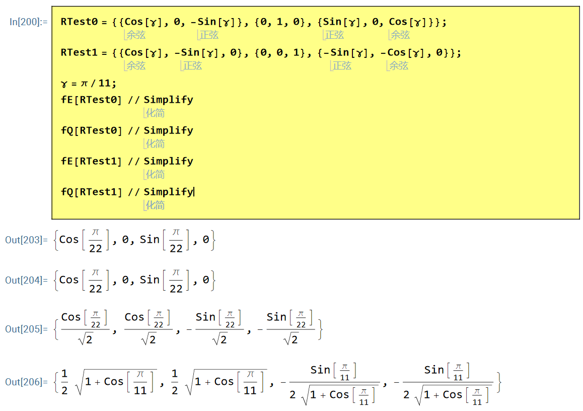
Example 1: IJSS 248 (2022) 111685
In this reference, the left and right local frames (row vector form) of the rod are defined as:
Left-end local frame $\mathbf{D}_0$:
\[\begin{pmatrix} \mathbf{d}_1^t \\ \mathbf{d}_2^t \\ \mathbf{d}_3^t \end{pmatrix} = \begin{pmatrix} \cos\gamma & 0 & -\sin\gamma \\ 0 & 1 & 0\\ \sin\gamma & 0 & \cos\gamma \end{pmatrix}\]Right-end local frame $\mathbf{D}_1$:
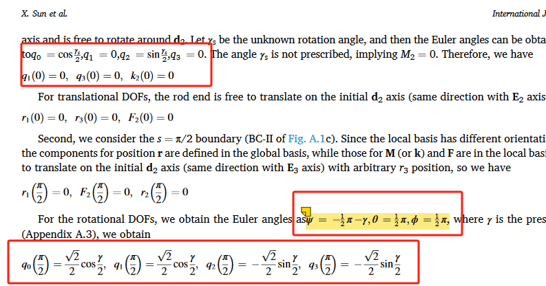
\[\begin{pmatrix} \mathbf{d}_1^t \\ \mathbf{d}_2^t \\ \mathbf{d}_3^t \end{pmatrix} = \begin{pmatrix} \cos\gamma & -\sin\gamma & 0 \\ 0 & 0 & 1\\ -\sin\gamma & -\cos\gamma & 0 \end{pmatrix}\]Treating the above frame matrices as rotation matrices $\mathbf{R}$ (note that this is row-vector form, corresponding to $\mathbf{R}^T$ in the derivation above) and substituting them into the Mathematica program above yields the boundary conditions consistent with the reference (initial values of quaternions $q_0, q_1, q_2, q_3$).
Schematic diagrams of the results are shown below:
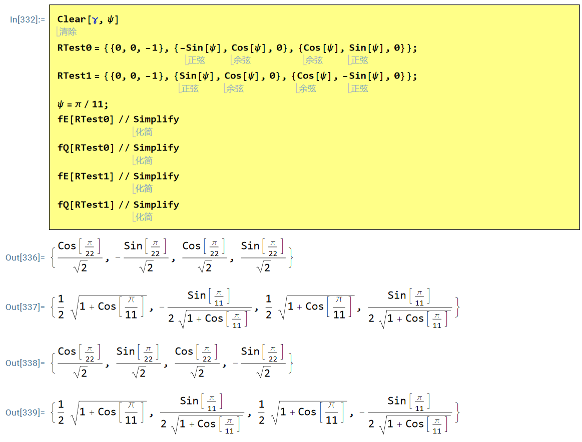
Example 2: JMPS 122 (2019) 657–685
In this reference, the left and right local frames (row vector form) of the rod are defined as:
Left-end local frame $\mathbf{D}_0$:
\[\left( \begin{matrix} \mathbf{d}_1^t \\ \mathbf{d}_2^t \\ \mathbf{d}_3^t \end{matrix} \right) = \left( \begin{matrix} 0 & 0 & -1 \\ -\sin\psi & \cos\psi & 0 \\ \cos\psi & \sin\psi & 0 \end{matrix} \right)\]Right-end local frame $\mathbf{D}_1$:
\[\begin{pmatrix} \mathbf{d}_1^t \\ \mathbf{d}_2^t \\ \mathbf{d}_3^t \end{pmatrix}=\begin{pmatrix} 0 & 0 & -1 \\ \sin\psi & \cos\psi & 0\\ \cos\psi & -\sin\psi & 0 \end{pmatrix}\]Similarly, substituting the above matrices into the Mathematica program yields the corresponding quaternion boundary conditions, consistent with the reference.
Schematic diagrams of the results are shown below: