
Notes for VASP
Published:
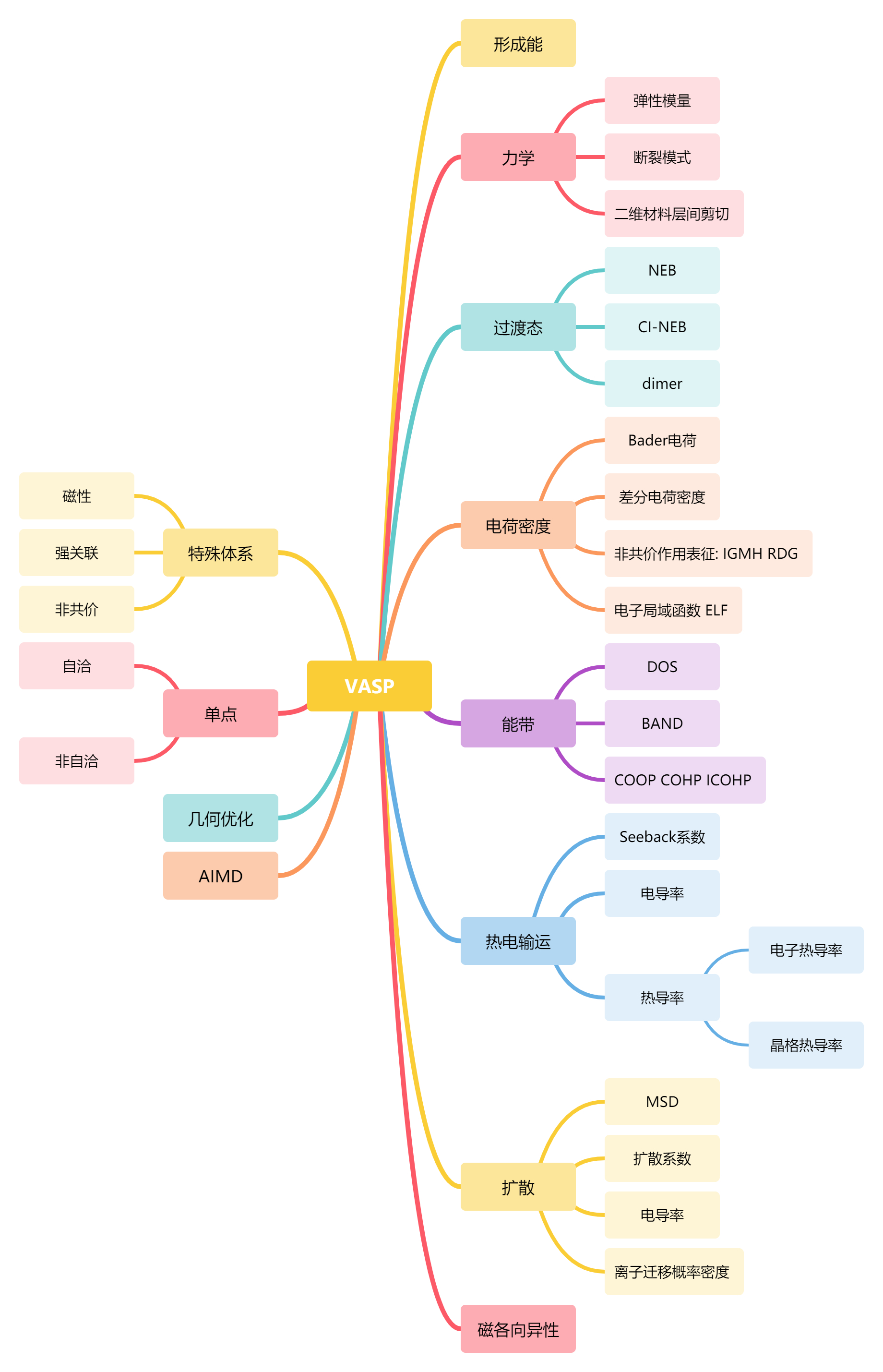
Summary of VASP calculation parameters.
Global
IO parameters - ISTART = 1 read wavefunction - ICHARG = 1 read charge density (11 for DOS and BAND) - LWAVE = .TRUE. write wavefunction - LCHARG = .TRUE. write charge density - LELF = .FALSE. write ELFCAR
Precision parameters
- ENCUT = 1.3*ENMAX in POTCAR - #NELECT = ? number of valence electrons (Background charge) - ADDGRID = .TRUE. oscillations the charge density - PREC = Accurate - LREAL = Auto projection done in real space
Parallel parameter - KPAR = number of cores/KPAR for one k-point - NCORE = cores/KPAR/NPAR -#NPAR =
SP
- ISMEAR = 0/1/-5
- SIGMA = 0.02~0.05/0.2/\
- NELM = 200
- EDIFF = 1e-5~1e-4
- # NEDOS = 2000
- # LORBIT = 11
OPT
- NSW = 2000
- IBRION = 2(CG) 0(MD) 3(CI-NEB)
- ISIF = 2 (ions) 3 (ions/shape)
- EDIFFG = -1e-2 ~ -5e-2 force smaller 0.02A/eV
- ISYM = 2 use symmetry 0 for AIMD
- ALGO = VeryFast (Normal for magnetic system)
MAGMOM
- ISPIN = 2 open spin 1 close spin
- MAGMOM = n1*uB1 n2*uB2 n1*uB1 n2*uB2 n3*uB3 n4*uB4
- VOSKOWN = 0 (1 for PW91 function)
- LASPH = .TRUE. (Non-spherical elements, d/f convergence)
- GGA_COMPAT = .FALSE. (Apply spherical cutoff on gradient field FALSE for magnetic anisotropy)
- AMIX = 0.2 (Mixing parameter to control SCF convergence)
- BMIX = 0.0001 (Mixing parameter to control SCF convergence)
- AMIX_MAG = 0.4 (Mixing parameter to control SCF convergence)
- BMIX_MAG = 0.0001 (Mixing parameter to control SCF convergence)
DFT+U
- LDAU = .TRUE. (Activate DFT+U)
- LMAXMIX = 4 (For d elements increase LMAXMIX to 4, f: LMAXMIX = 6)
- LDAUTYPE = 2 (Dudarev, only U-J matters)
- LDAUL = d/f d/f d/f d/f (Orbitals for each species 1p 2d 3f -1none)
- LDAUU = U1 U2 U3 U4
- LDAUJ = 0 0 0 0
NEB
- ICHAIN = 0 (Open NEB)
- LCLIMB = .TRUE. (Choose CI-NEB)
- IOPT = 1/2/7 (7:Fast Inertial Relaxation Engine; 2:CG)
- POTIM = 0 (Use method provided by CI-NEB)
- IMAGES = 8 (Numbers of interpolation points)
- SPRING = -5 (Spring force)
Parameters to set for different systems
- System properties: SIGMA; ISMEAR; DFT+U; MAGMOM
- Convergence parameters: EDIFF; EDIFFG; NSW; NELM
- Non-self-consistent calculations: ICHARG; NEDOS; LORBIT
- Parallel parameters: NCORE; KPAR
Free energy correction
NFREE = 2 IBRION = 0.015
Automation scripts - Optimization + single point - Single point + non-self-consistent band - Free energy correction
Experience summary - liujc
I personally usually perform stepwise structure optimization. In the first step of structure optimization, use lower precision while setting ISMEAR = 0 + SIGMA = 0.1. Check the EENTRO value given at the end of the optimization in the OUTCAR file. Then determine whether the system is a semiconductor or metal by dividing the EENTRO value by the number of atoms:
1) (EENTRO / number of atoms) > 1 meV, the system is a metal.
2) (EENTRO / number of atoms) < 0.1 meV, the system is a semiconductor. When this value is very small, e.g., 0.000001, the band gap is generally large.
3) (EENTRO / number of atoms) between 1 meV and 0.1 meV, not specifically tested yet, uncertain.
The basis for this judgment is: for metallic systems, ISMEAR = 0 uses Gaussian smearing, which leads to fractional occupations at the Fermi level, causing the EENTRO value to be non-zero. For semiconductors with large band gaps, SIGMA = 0.1 cannot yet cause fractional occupations at the Fermi level, so EENTRO remains 0 (if SIGMA is increased to a very large value, EENTRO will no longer stay 0, but the calculation will be problematic).
This judgment method is based on my personal experience. It has provided correct results in most cases so far, but I cannot guarantee it works for all systems under all conditions. For example, when the lattice changes significantly during relaxation, the plane wave cutoff sphere used for self-consistent calculations may become severely distorted, potentially causing the ionic step’s self-consistent convergence to converge to a state with significant errors. I’m unsure whether this method can still be reliably applied under such erroneous self-consistent results. However, the solution is simple: perform another relaxation using the relaxed structure, and then this method can be applied.
Bader Charge Calculations
## What is Bader charge?
In a molecule, charge is not uniformly distributed throughout the space occupied by the molecule. Between every two atoms, the charge density distribution is non-uniform, and the charge density increases significantly closer to the atoms. Therefore, there exists a minimum between two larger values, and this minimum is the dividing line between atoms. The minimum points around an atom form a closed region that can be used to partition atoms within the molecule. The integrated charge within this region is the Bader charge. (VASP uses pseudopotentials, so the total calculated charge is the sum of all “valence” electrons in the current chemical environment.)
## Bader charge calculation
Bader is software for calculating Bader charges. It reads two types of input files:
1 VASP CHGCAR file;
2 Gaussian CUBE file. The software automatically recognizes the file format without manual specification.
Usage
Bader filename
Options are listed in the table below:
| Option | Meaning |
|---|---|
| -c bader | voronoi | Enable Bader calculation / Voronoi polyhedron calculation |
| -n bader | voronoi | Disable Bader calculation / Voronoi polyhedron calculation |
| -b neargrid | ongrid | weight | Three Bader grid partitioning algorithms |
| -r refine_edge_method | Default -1, generally use -1 (new algorithm, efficient; old algorithm is -2) |
| -ref reference_charge | Reference charge (-ref file(AECCAR0+AECCAR2) recommended) |
| -vac off | auto | vacuum_density | Default specifies low-density points for vacuum layer (1e-3/A^3 criteria) |
| -p all_atom | all_bader | Output options |
| -p sel_atom | sel_bader | Output options (selection) |
| -p sum_atom | sum_bader | Output options (summation) |
| -p atom_index | bader_index | Output options (index) |
| -i cube | chgcar | Default is auto-detect, generally do not set! |
| -cp | Select critical points |
| -h | Help |
| -v | Verbose output |
Output files:
| File name | Content |
|---|---|
| ACF.dat | Coordinates, charge, minimum distance to surface (inner layer), volume |
| BCF.dat | Coordinates, charge, nearest atom, distance to nearest atom |
| AVF.dat | Volume |
Crude approach:
Ignore core electrons and use the pseudopotential’s core electron count (generally core electrons do not change much)
bader CHGCAR
Officially recommended approach:
Consider core electrons, consider full electron state
LAECHG =.TRUE. LCHARG = .TRUE. NSW = 0
chgsum.pl AECCAR0 AECCAR2 bader CHGCAR -ref CHGCAR_sum