The Elastic Rod Problem and Its Numerical Solution

What shape does a rope take when subjected to forces, bending moments, and torques?

• Preliminary work
• Formulating the Euler elastic rod equation
• Analytical solution
• Numerical solution
• Elastic rods in Riemannian space
• Appendix: C++ code

Preliminary Work

The Magic of Integration by Parts

In A Brief Discussion of Integration by Parts, iteration was used to obtain:

Using this formula, the higher-order Lagrange equation was also derived. Here is a brief summary for later use:

The Lagrange equation with higher-order derivatives is:

The corresponding conserved quantity is:

A Few Elliptic Functions

Just some symbolic transformations.

Formulating the Euler Elastic Rod Equation

When the elastic rod is inextensible, the energy can be written as:

This inextensibility assumption has physical meaning independent of a large elastic modulus. For example, consider a relaxed curved rubber band: even though rubber is easily stretched, if the rope is not taut, it can be treated as inextensible for bending energy purposes.

When rotation is not considered, the energy is contributed only by curvature.

The relation between curvature and the position vector is:

Using the Lagrange multiplier method, the energy functional becomes:

Applying the second-order Lagrange equation derived above gives:

The conserved quantity is:

The above expresses the relation that the position vector must satisfy. To connect the position vector with the intrinsic quantities of the curve (what are intrinsic quantities? They are properties inherent to the system, independent of coordinate choice — here, curvature and torsion), we need to project the position vector onto the Frenet frame (not necessarily the Frenet frame; any frame attached to the curve will do) and simplify using the Frenet relations.

(Add: How to understand intrinsic coordinates? First, for a space curve, choosing different base points yields different parametric equations for the position vector. However, $r’(s)$ is independent of the choice of base point. This also explains why the Frenet frame, which describes the curve’s own properties, does not contain $r$, but only the derivatives of $r$.)

The Frenet relations:

After projection (skipping lengthy algebra):

All three components must vanish:

Integrating the above:

The next step is simply to solve the equation using boundary conditions, then map the parameter space $(\kappa,\tau,s)$ to Euclidean space $(x,y,z)$.

Analytical Solution

???????????????????????

Numerical Solution

In the elastic rod problem, it is convenient to solve using intrinsic parameters. However, for visualization, a coordinate transformation from the intrinsic parameter space to Euclidean space is necessary. This transformation involves solving the Frenet equations.

Key to numerical solution: Solve the Frenet equations to transform the parameter space into Euclidean space.

First, consider the two-dimensional case as shown below:

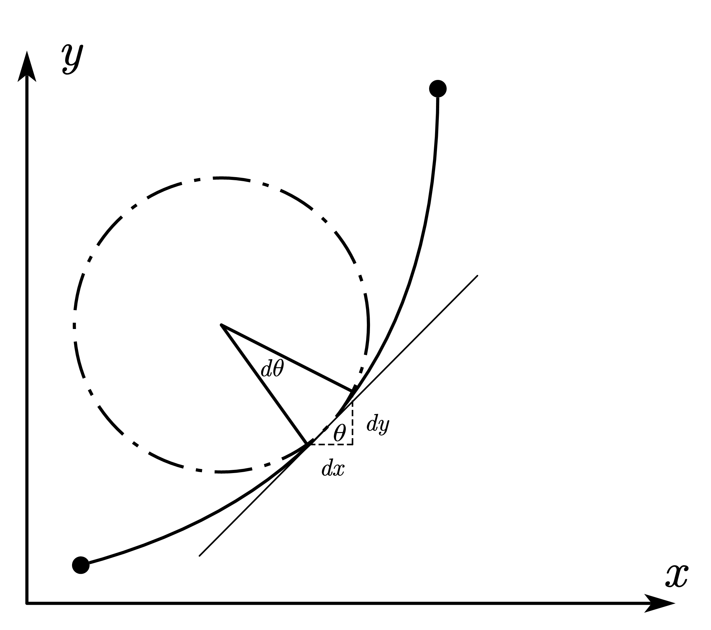
At first glance it seems very simple. Quickly, the transformation between the parameter space and Euclidean space can be written down from geometric intuition.

Discretization:

But what is the geometric relation in three dimensions?

That is, when moving a distance $ds$ from a point $(x_0,y_0,z_0)$ on the curve, with both bending and twisting occurring, how do we express the new position?

It becomes difficult to obtain this relation through geometric intuition alone, as in the two-dimensional case.

Thus, we realize that the above “geometric intuition” transformation is simply a parameterization using an intermediate parameter $\theta$.

Can we do the same in three dimensions?

Parameterize the arc length as:

How do we relate $(\theta,\varphi)$ to the intrinsic parameters?

Using the Frenet equations:

At this point, if we can find the relation between $(\kappa,\tau)$ and $(\theta,\phi)$, we can transform the parameter space into Euclidean space. However, this is a complex nonlinear equation that is difficult to discretize, so this approach does not work.

We took a long detour and ended up in a dead end.

Since the parameter space transformation is related to the Frenet equations, why not solve the Frenet equations directly?

How do we map the Frenet equations to Euclidean space?

Through the relation $T(s)=r’(s)$.

Now we have a clear solution approach. This thought process is quite interesting.

Perhaps the detour was not a waste. The geometric intuition from the 2D case led us to think about the 3D case. When geometric intuition failed in 3D, we had to go back and generalize the 2D approach. After generalizing, we found the same method could not solve the 3D problem. At that point, we realized the difference: the Frenet equations are used in 3D. This led us to the Frenet equations, and ultimately to solving them — obtaining a general method for transforming from the parameter space to Euclidean space.

Discretizing the Frenet equations and $T=r’(s)$:

Thus, the solution approach for the Euler elastic rod (considering only bending energy) is summarized as:

1. Solve the elastic rod equation \(\kappa'' \left( s \right) +\frac{1}{2}\kappa ^3\left( s \right) -\frac{\lambda}{2}\kappa \left( s \right) -\frac{c^2}{\kappa^3\left( s \right)}=0\)
2. Obtain the evolution of intrinsic parameters $(\kappa(s),\tau(s))$
3. Solve for the evolution of the $(T,N,B)$ frame via the Frenet equations
4. Map the parameter space to Euclidean space via $r’(s)=T$

PS: The above is a second-order equation for curvature. It can be solved by iteration given initial curvature and its derivative (initial value problem), or by shooting method given boundary conditions at two endpoints (boundary value problem). Additionally, the Euler method produces large errors when solving the Frenet equations (even for a simple circle), whereas a predictor-corrector algorithm performs much better.

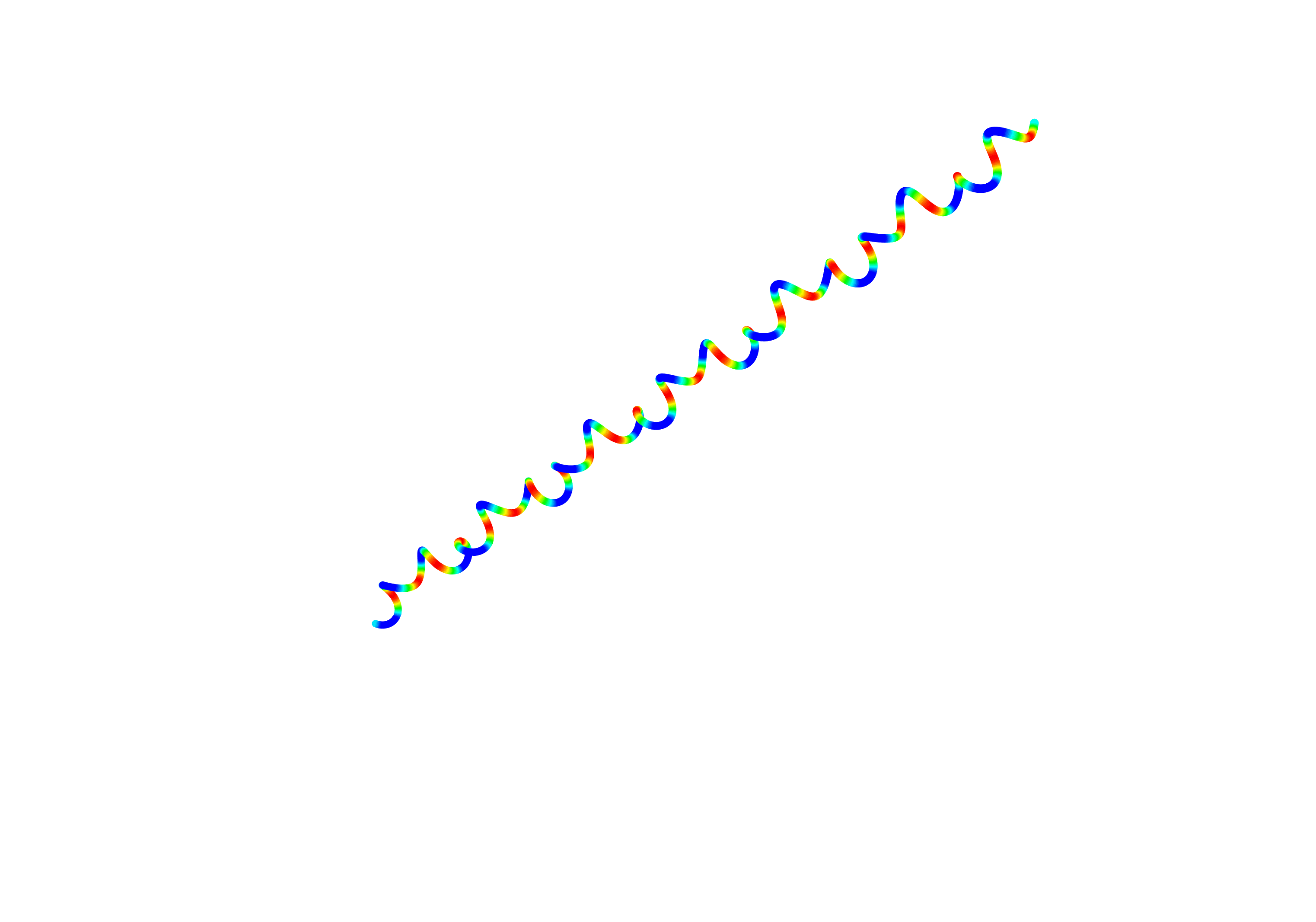
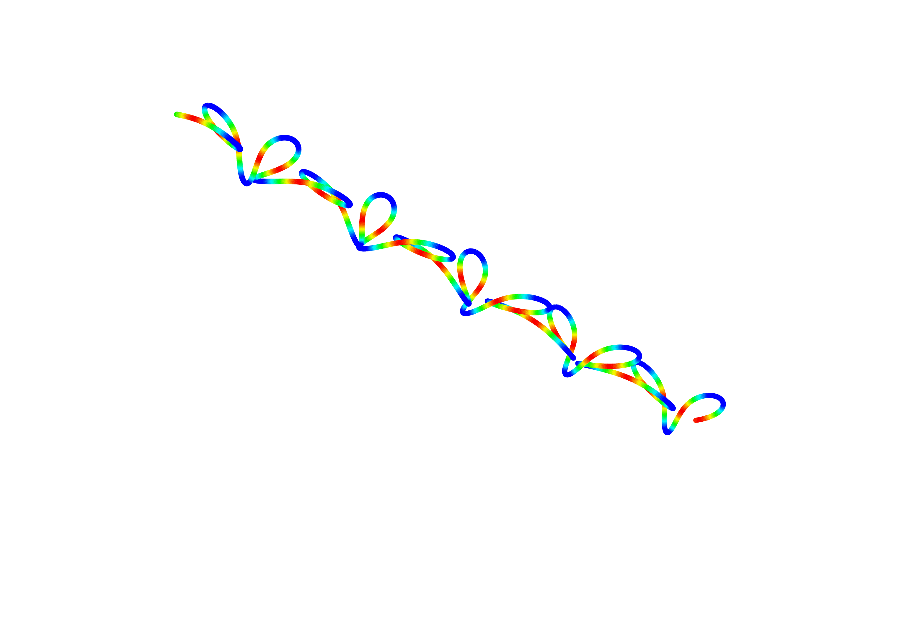
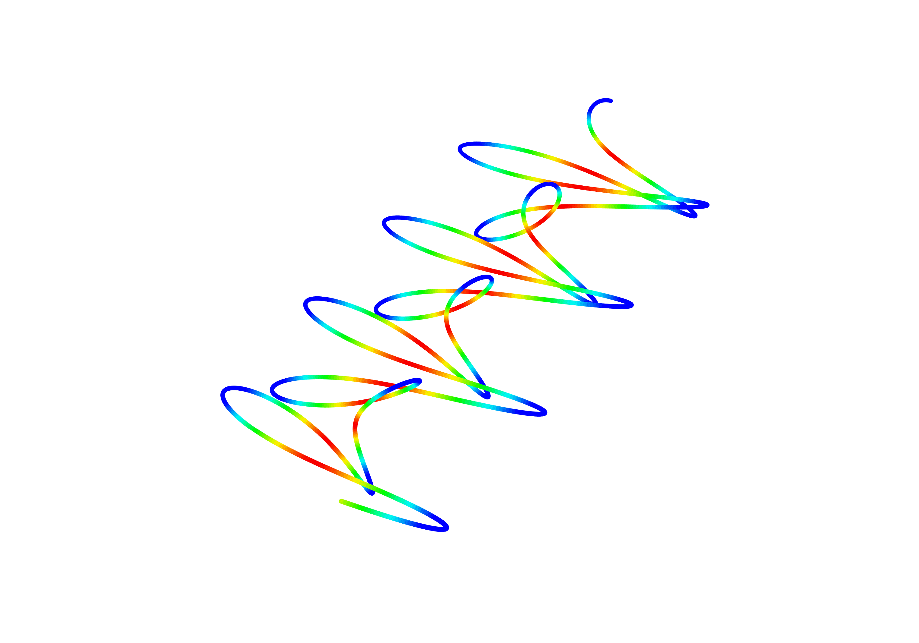
The solution method is already given above. Below are visualizations of several solutions (colored by curvature):

Elastic Rods in Riemannian Space

???????????????????????

C++ Code

Main function (main.cpp):

#############Elastica类(EulerElasticaRod.h)#############
#include<iostream>
#include<fstream>
#include<math.h>
using namespace std;
struct Para{
	static const int N=2000;
	double kappa[N]{},tau[N]{},coord[3][N];
};
class DER{
public:
	//	Para ks2coord();
	DER(Para &p1,double s1,double* kppa01,double k01,double dk01,double tau0,double ks,double lambda1);//构造函数
	//不需要析构函数！！
	Para SolveER();
	double erfen();
	double f();
	double f1();
private:
	Para p;double s;double* kppa0;double k0;double dk0;double tau0;double ks;double lambda;	
};
DER::DER(Para &p1,double s1,double* kppa01,double k01,double dk01,double tau01,double ks0,double lambda1){
	p=p1;s=s1;kppa0=kppa01;k0=k01;dk0=dk01;ks=ks0;lambda=lambda1;tau0=tau01;
}
//就是不需要析构函数！！！
//定义public函数
Para DER::SolveER(){
	int NN=p.N; 
	double ds=s/NN;
	double c=k0*k0*tau0;
	p.kappa[0]=k0;p.kappa[1]=ds*dk0+k0;p.tau[0]=tau0;
	for (int i =1;i<NN-1;i++) 
	{
		p.kappa[i+1]=2*p.kappa[i]-p.kappa[i-1]+pow(ds,2)*(-0.5*pow(p.kappa[i],3)+0.5*lambda*p.kappa[i]+pow(c,2)/pow(p.kappa[i],3));
		p.tau[i+1]=c/pow(p.kappa[i+1],2);
	}
	return p;	
} 


double DER::erfen(){
	cout<<"ks"<<"         "<<"err"<<endl;
	double ff0=this->f();double ff1=this->f1();
	double eps=1e-6;
	
	while(true){
		dk0=dk0-(ff0-ks)/ff1;
		ff0=DER(p,s,kppa0,k0,dk0,tau0,ks,lambda).f();
		ff1=DER(p,s,kppa0,k0,dk0,tau0,ks,lambda).f1();
		cout<<ff0<<"    "<<abs(ff0-ks)<<endl;
		if (abs(ff0-ks)<eps) break;	
	}
	return dk0;	
}
double DER::f(){
	Para re=SolveER();
	return re.kappa[re.N-1];
}
double DER::f1(){
	double ddk=0.001;
	return (DER(p,s,kppa0,k0,dk0+ddk,tau0,ks,lambda).f()-DER(p,s,kppa0,k0,dk0,tau0,ks,lambda).f())/ddk;
}


#############主函数#############
#include "EulerElasticaRod.h"
Para ks2coord(Para &p, double s) {
	double Frenet[3][p.N][3] {}, ds = s / p.N;
	Frenet[0][0][0] = 1;
	Frenet[0][0][1] = 0;
	Frenet[0][0][2] = 0;
	Frenet[1][0][0] = 0;
	Frenet[1][0][1] = 1;
	Frenet[1][0][2] = 0;
	Frenet[2][0][0] = 0;
	Frenet[2][0][1] = 0;
	Frenet[2][0][2] = 1;
	for (int j = 0; j < 3; j++) {
		p.coord[j][0] = 0;
		for (int i = 1; i < p.N; i++) {
			Frenet[0][i][j] = Frenet[0][i - 1][j] + p.kappa[i - 1] * ds * Frenet[1][i - 1][j];
			Frenet[2][i][j] = Frenet[2][i - 1][j] - p.tau[i - 1] * ds * Frenet[1][i - 1][j];
			Frenet[1][i][j] = Frenet[1][i - 1][j] - p.kappa[i - 1] * ds * Frenet[0][i - 1][j] + p.tau[i - 1] * ds * Frenet[2][i - 1][j];
			//预报校正算法 PS:简单的Euler法会导致比较大的误差，不信试试看！
			Frenet[0][i][j] = Frenet[0][i - 1][j] + p.kappa[i - 1] * ds * (Frenet[1][i - 1][j] + Frenet[1][i][j]) / 2;
			Frenet[2][i][j] = Frenet[2][i - 1][j] - p.tau[i - 1] * ds * (Frenet[1][i - 1][j] + Frenet[1][i][j]) / 2;
			Frenet[1][i][j] = Frenet[1][i - 1][j] - p.kappa[i - 1] * ds * (Frenet[0][i - 1][j] + Frenet[0][i][j]) / 2 + p.tau[i - 1] * ds * (Frenet[2][i - 1][j] + Frenet[2][i][j]) / 2;
			p.coord[j][i] = p.coord[j][i - 1] + Frenet[0][i - 1][j] * ds;
		}
	}
	return p;
}
int main() {
	Para p;
	double s = 50, kappa[p.N] {}, k0 = 0.9, dk0 = 0.9, tau0 = 1, lambda = 0.75, ks = 2;
	double ppp = DER(p, s, kappa, k0, dk0, tau0, ks, lambda).erfen();
	Para q = DER(p, s, kappa, k0, ppp, tau0, ks, lambda).SolveER();
	//	dk0=DER(p,s,kappa,k0,dk0,tau0,ks,lambda).erfen();
	Para ret = ks2coord(q, s);
	cout << ret.kappa[q.N - 1] << endl;
	ofstream out("out.data");
	for (int i = 0; i < p.N; i++) {
		out << ret.coord[0][i] << "   " << ret.coord[1][i] << "   " << ret.coord[2][i]<<"    "<<ret.kappa[i]<< endl;
	}
	out.close();
	return 0;
}