
Some Fragmented Mathematical Notes
Published:
Some fragmented mathematical notes.
Geometry
Notes on Classical Curve Theory
Classical differential geometry often introduces curve theory via the Frenet frame (geometrically intuitive). But how can we view curve theory from the perspective of tensors?
Definitions
A frame is a set of vectors ${ \mathbf{e}_1, \mathbf{e}_2, \mathbf{e}_3 }$ satisfying
\[\begin{cases} \frac{d\mathbf{e}_i}{ds} = \Gamma_i^{\,j}\mathbf{e}_j, \\ \mathbf{e}_i \cdot \mathbf{e}_j = \delta_{ij}. \end{cases}\]Properties
The following properties can be derived from the above equations.
1. $\Gamma_j^{\,i} + \Gamma_i^{\,j} = 0$
\[\frac{d}{ds}\left( \mathbf{e}_i \cdot \mathbf{e}_j \right) = \mathbf{e}_i \cdot \frac{d\mathbf{e}_j}{ds} + \frac{d\mathbf{e}_i}{ds} \cdot \mathbf{e}_j = \Gamma_j^{\,i} + \Gamma_i^{\,j} = 0.\]2. Relations among ${ \Omega, \omega, \Gamma }$
\[\frac{d\mathbf{e}_j}{ds} = \mathbf{\omega} \times \mathbf{e}_j = \mathbf{\Omega} \cdot \mathbf{e}_j.\] \[\mathbf{e}_i \times \frac{d\mathbf{e}_i}{ds} = \mathbf{e}_i \times \left( \mathbf{\omega} \times \mathbf{e}_i \right) = 3\mathbf{\omega} - \omega_i \mathbf{e}_i = 2\mathbf{\omega} = \epsilon_{ijk}\Gamma_i^{\,j}\mathbf{e}_k.\]Therefore
\[\mathbf{\omega} = \frac{1}{2}\epsilon_{ijk}\Gamma_i^{\,j}\mathbf{e}_k.\]For the Frenet frame:
\[\mathbf{\omega} = \kappa \mathbf{e}_3 + \tau \mathbf{e}_1.\]For the Bishop frame:
\[\mathbf{\omega} = \kappa_1 \mathbf{b}_2 - \kappa_2 \mathbf{b}_1.\]If $\mathbf{\Omega} \cdot \mathbf{a} = \mathbf{\omega} \times \mathbf{a}$, then
\[\begin{cases} \frac{1}{2}\mathbf{\epsilon} : \mathbf{\Omega} + \mathbf{\omega} = 0, \\ \mathbf{\epsilon} \cdot \mathbf{\omega} + \mathbf{\Omega} = 0. \end{cases}\]Combining the above expressions:
\[\Omega_{ij} = -\frac{\epsilon_{ijk}\epsilon_{ijk}\Gamma_i^{\,j}}{2} = -\delta_{kk}\Gamma_i^{\,j} = -\Gamma_i^{\,j}.\]Note that $\delta$ is not summed here.
We obtain the following conclusion:
\[\begin{cases} \mathbf{\Omega} + \mathbf{\Gamma} = 0, \\ \mathbf{\Gamma} = \mathbf{\epsilon} \cdot \mathbf{\omega}, \\ \mathbf{\omega} = \dfrac{1}{2}\mathbf{\epsilon} : \mathbf{\Gamma}, \\ \dfrac{1}{2}\mathbf{\epsilon} : \mathbf{\Omega} + \mathbf{\omega} = 0, \\ \mathbf{\epsilon} \cdot \mathbf{\omega} + \mathbf{\Omega} = 0. \end{cases}\]It can be seen that the Darboux vector and the rotation tensor $\mathbf{\Omega}$ are entirely induced by $\mathbf{\Gamma}$ and $\mathbf{\epsilon}$.
Thus the Frenet equations determine the intrinsic structure of a curve.
3. Relations among Bishop, Frenet, and Material frames
\[\begin{cases} \frac{d\mathbf{e}_i}{ds} = \Gamma_i^{\,j}\mathbf{e}_j, \\ \mathbf{e}_i \cdot \mathbf{e}_j = \delta_{ij}. \end{cases}\]Consider $\mathbf{p}_i = R_i^{\,j}\mathbf{e}_j$, i.e., a rotation between reference frames.
\[\frac{d\mathbf{p}_i}{ds} = \Gamma_i^{\,j}\mathbf{p}_j = \Gamma_i^{\,j} R_j^{\,m}\mathbf{e}_m = \frac{dR_i^{\,m}}{ds}\mathbf{e}_m + R_i^{\,m}\frac{d\mathbf{e}_m}{ds} = \frac{dR_i^{\,m}}{ds}\mathbf{e}_m + R_i^{\,j}{\Gamma_0}_j^{\,m}\mathbf{e}_m.\] \[\frac{d\mathbf{p}_i}{ds} \cdot \mathbf{p}_j = \Gamma_i^{\,j} = \frac{dR_i^{\,m}}{ds}R_j^{\,m} + R_i^{\,n}{\Gamma_0}_n^{\,m}R_j^{\,m}.\]Obtaining the important expression:
\[\Gamma_i^{\,j} = \frac{dR_i^{\,m}}{ds}R_j^{\,m} + R_i^{\,n}{\Gamma_0}_n^{\,m}R_j^{\,m}.\]Consider the rotation and the three types of frames:
\[R = \begin{bmatrix} 1 & 0 & 0 \\ 0 & \cos\theta & \sin\theta \\ 0 & -\sin\theta & \cos\theta \end{bmatrix},\] \[\frac{dR}{ds} = \begin{bmatrix} 0 & 0 & 0 \\ 0 & -\sin\theta & \cos\theta \\ 0 & -\cos\theta & -\sin\theta \end{bmatrix} \theta'(s).\]The connection matrices of the three frames are:
\[\text{Bishop}\; \begin{bmatrix} 0 & \kappa_1 & \kappa_2 \\ -\kappa_1 & 0 & 0 \\ -\kappa_2 & 0 & 0 \end{bmatrix}, \qquad \text{Frenet}\; \begin{bmatrix} 0 & \kappa & 0 \\ -\kappa & 0 & \tau \\ 0 & -\tau & 0 \end{bmatrix}, \qquad \text{Material}\; \begin{bmatrix} 0 & m_1 & m_2 \\ -m_1 & 0 & m \\ -m_2 & -m & 0 \end{bmatrix}.\]From the above tensor equations:
Rotating the Bishop frame about the $\mathbf{e}_1$ axis by $\theta$ gives the Frenet frame, where $\theta$ satisfies
\[\begin{cases} \kappa = \kappa_1 \cos\theta + \kappa_2 \sin\theta, \\ \kappa_1 \sin\theta = \kappa_2 \cos\theta, \\ \theta' = \tau. \end{cases}\]Rotating the Bishop frame about the $\mathbf{e}_1$ axis by $\theta$ gives the Material frame, where $\theta$ satisfies
\[\begin{cases} m_1 = \kappa_1 \cos\theta + \kappa_2 \sin\theta, \\ m_2 = -\kappa_1 \sin\theta + \kappa_2 \cos\theta, \\ m = \theta'. \end{cases}\]Rotating the Frenet frame about the $\mathbf{e}_1$ axis by $\theta$ gives the Material frame, where $\theta$ satisfies
\[\begin{cases} m_1 = \kappa \cos\theta, \\ m_2 = -\kappa \sin\theta, \\ m = \theta' + \tau. \end{cases}\]Notes on Classical Surface Theory
Fundamental Forms of a Surface
Consider a surface parametrized by $\mathbf{r}(u,v)$. The line element is written as
\[\mathrm{I} = d\mathbf{r} \cdot d\mathbf{r} = \mathbf{r}_u \cdot \mathbf{r}_u\,du^2 + 2\mathbf{r}_u \cdot \mathbf{r}_v\,du\,dv + \mathbf{r}_v \cdot \mathbf{r}_v\,dv^2 = E\,du^2 + 2F\,du\,dv + G\,dv^2.\]This is called the first fundamental form.
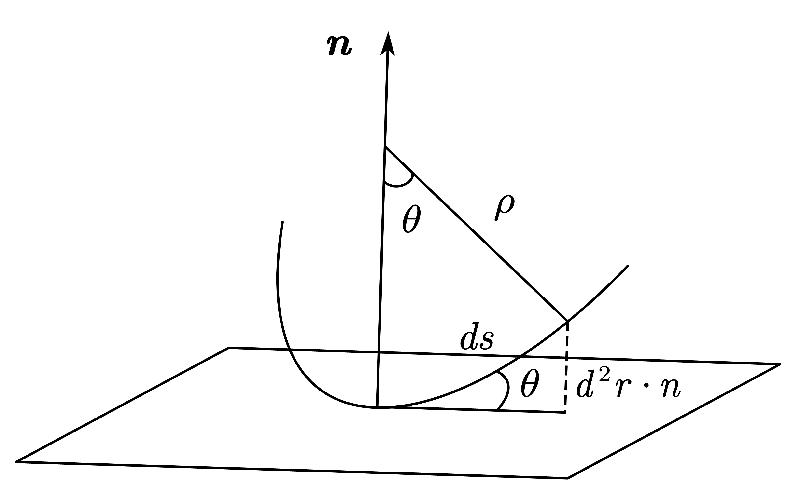
From the geometric relations in the figure:
\[\theta\,ds = \frac{1}{\rho}ds^2 = \kappa_n\,d\mathbf{r} \cdot d\mathbf{r} = \kappa_n \mathrm{I} = d^2\mathbf{r} \cdot \mathbf{n}.\]Define $d^2\mathbf{r} \cdot \mathbf{n} = \mathrm{II}$ as the second fundamental form.
\[\mathrm{II} = d^2\mathbf{r} \cdot \mathbf{n} = \left( \partial_u\,du + \partial_v\,dv \right)^2 \mathbf{r} \cdot \mathbf{n} = \mathbf{r}_{uu}\cdot \mathbf{n}\,du^2 + 2\mathbf{r}_{uv}\cdot \mathbf{n}\,du\,dv + \mathbf{r}_{vv}\cdot \mathbf{n}\,dv^2 = L\,du^2 + 2M\,du\,dv + N\,dv^2.\]The normal curvature $\kappa_n$ is expressed as
\[\kappa_n = \frac{\mathrm{II}}{\mathrm{I}}.\]Summary:
\[\begin{cases} E = \mathbf{r}_u \cdot \mathbf{r}_u, \\ F = \mathbf{r}_u \cdot \mathbf{r}_v, \\ G = \mathbf{r}_v \cdot \mathbf{r}_v, \\ L = \mathbf{r}_{uu} \cdot \mathbf{n} = -\mathbf{r}_u \cdot \mathbf{n}_u, \\ M = \mathbf{r}_{uv} \cdot \mathbf{n} = -\mathbf{r}_u \cdot \mathbf{n}_v = -\mathbf{r}_v \cdot \mathbf{n}_u, \\ N = \mathbf{r}_{vv} \cdot \mathbf{n} = -\mathbf{r}_v \cdot \mathbf{n}_v, \\ \kappa_n = \dfrac{\mathrm{II}}{\mathrm{I}} = \dfrac{L\,du^2 + 2M\,du\,dv + N\,dv^2}{E\,du^2 + 2F\,du\,dv + G\,dv^2}. \end{cases}\]Clearly $\dfrac{du}{dv}$ determines the direction of normal curvature on the surface.
Principal Curvature, Mean Curvature, Gaussian Curvature
Focusing on the extremum of normal curvature, let $du/dv = p$, then
\[\left( \kappa_n E - L \right)p^2 + 2\left( \kappa_n F - M \right)p + \kappa_n G - N = 0.\]For a quadratic equation to have a solution, $\Delta \ge 0$, therefore
\[(EG - F^2)\kappa_n^2 - (EN - 2FM + GL)\kappa_n + LN - M^2 \le 0.\]By the Cauchy inequality we always have
\[(\mathbf{r}_u \cdot \mathbf{r}_v)^2 \le |\mathbf{r}_u|^2 |\mathbf{r}_v|^2,\]i.e., $F^2 \le EG$. The quadratic coefficient is positive, the quadratic form is negative, and $\kappa_n$ is bounded between the two roots.
The maximum and minimum principal curvatures are
\[\begin{cases} \kappa_1 = \dfrac{ (EN - 2FM + GL) + \sqrt{(EN - 2FM + GL)^2 - 4(F^2 - EG)(M^2 - LN)} }{ 2(EG - F^2) }, \\[1.2em] \kappa_2 = \dfrac{ (EN - 2FM + GL) - \sqrt{(EN - 2FM + GL)^2 - 4(F^2 - EG)(M^2 - LN)} }{ 2(EG - F^2) }, \\[1.2em] \dfrac{\kappa_1 + \kappa_2}{2} = \dfrac{EN - 2FM + GL}{2(EG - F^2)}, \\[1.2em] \kappa_1 \kappa_2 = \dfrac{LN - M^2}{EG - F^2}. \end{cases}\]where
\[K = \kappa_1 \kappa_2\]is called the Gaussian curvature, and
\[H = \frac{\kappa_1 + \kappa_2}{2}\]is called the mean curvature.
Gauss Theorem Egregium
\[\begin{cases} L = \dfrac{\langle \mathbf{r}_{uu}, \mathbf{r}_u, \mathbf{r}_v \rangle}{EG - F^2}, \\ M = \dfrac{\langle \mathbf{r}_{uv}, \mathbf{r}_u, \mathbf{r}_v \rangle}{EG - F^2}, \\ N = \dfrac{\langle \mathbf{r}_{vv}, \mathbf{r}_u, \mathbf{r}_v \rangle}{EG - F^2}. \end{cases}\]The determinant of the second fundamental form can be written as
\[LN - M^2 = \det \begin{bmatrix} \mathbf{r}_{uu}\cdot \mathbf{r}_{vv} & \dfrac{E_u}{2} & F_u - \dfrac{E_v}{2} \\ F_v - \dfrac{G_u}{2} & E & F \\ \dfrac{G_v}{2} & F & G \end{bmatrix} - \det \begin{bmatrix} \mathbf{r}_{uv}\cdot \mathbf{r}_{uv} & \dfrac{E_v}{2} & \dfrac{G_u}{2} \\ \dfrac{E_v}{2} & E & F \\ \dfrac{G_u}{2} & F & G \end{bmatrix}.\]This can be further transformed to
\[LN - M^2 = \det \begin{bmatrix} F_{uv} - \dfrac{E_{vv} + G_{uu}}{2} & \dfrac{E_u}{2} & F_u - \dfrac{E_v}{2} \\ F_v - \dfrac{G_u}{2} & E & F \\ \dfrac{G_v}{2} & F & G \end{bmatrix} - \det \begin{bmatrix} 0 & \dfrac{E_v}{2} & \dfrac{G_u}{2} \\ \dfrac{E_v}{2} & E & F \\ \dfrac{G_u}{2} & F & G \end{bmatrix}.\]Therefore, the Gaussian curvature depends only on the first fundamental form (the metric of the surface), meaning that when the surface does not stretch (dominated by bending energy), the Gaussian curvature is invariant.
Structure Equations of a Surface
Similar to the Frenet frame, considering $\mathbf{n}$ as the unit normal vector (perpendicular to the tangent plane), the structure equations of a surface can be written as
\[\begin{cases} \partial_\alpha \mathbf{r} = \mathbf{r}_\alpha, \\ \mathbf{r}_{\alpha\beta} = \Gamma_{\alpha\beta}^{\,\gamma} \mathbf{r}_\gamma + b_{\alpha\beta} \mathbf{n}, \\ \mathbf{n}_\alpha = -b_\alpha^{\,\gamma} \mathbf{r}_\gamma. \end{cases}\]It can be seen that $b$ is the coefficient of the second fundamental form.
Considering the commutativity of partial derivatives, first for $\mathbf{n}$:
\[\mathbf{n}_{\alpha\beta} = \mathbf{n}_{\beta\alpha}.\]Thus
\[\left( b_{\alpha\beta}^{\,\gamma} + b_\alpha^{\,\xi}\Gamma_{\xi\beta}^{\,\gamma} \right) \mathbf{r}_\gamma + b_\alpha^{\,\xi} b_{\xi\beta} \mathbf{n} = \left( b_{\beta\alpha}^{\,\gamma} + b_\beta^{\,\xi}\Gamma_{\xi\alpha}^{\,\gamma} \right) \mathbf{r}_\gamma + b_\beta^{\,\xi} b_{\xi\alpha} \mathbf{n}.\]Comparing coefficients gives
\[\begin{cases} b_{\alpha\beta}^{\,\gamma} + b_\alpha^{\,\xi}\Gamma_{\xi\beta}^{\,\gamma} = b_{\beta\alpha}^{\,\gamma} + b_\beta^{\,\xi}\Gamma_{\xi\alpha}^{\,\gamma}, \\ b_\alpha^{\,\xi} b_{\xi\beta} = b_\beta^{\,\xi} b_{\xi\alpha}. \end{cases}\]The second equation is automatically satisfied, and the first is called the Codazzi equation.
For $\mathbf{r}$:
\[\mathbf{r}_{\alpha\beta\gamma} = \Gamma_{\alpha\beta,\gamma}^{\,\xi}\mathbf{r}_\xi + b_{\alpha\beta,\gamma}\mathbf{n} + \Gamma_{\alpha\beta}^{\,p}\Gamma_{p\gamma}^{\,\xi}\mathbf{r}_\xi + \Gamma_{\alpha\beta}^{\,p} b_{p\gamma} \mathbf{n} - b_{\alpha\beta} b_\gamma^{\,\xi} \mathbf{r}_\xi.\]From $\mathbf{r}{\alpha\beta\gamma} = \mathbf{r}{\alpha\gamma\beta}$, comparing coefficients gives
\[\begin{cases} \Gamma_{\alpha\beta,\gamma}^{\,\xi} + \Gamma_{\alpha\beta}^{\,p}\Gamma_{p\gamma}^{\,\xi} - b_{\alpha\beta} b_\gamma^{\,\xi} = \Gamma_{\alpha\gamma,\beta}^{\,\xi} + \Gamma_{\alpha\gamma}^{\,p}\Gamma_{p\beta}^{\,\xi} - b_{\alpha\gamma} b_\beta^{\,\xi}, \\[0.6em] \Gamma_{\alpha\beta}^{\,p} b_{p\gamma} + b_{\alpha\beta,\gamma} = \Gamma_{\alpha\gamma}^{\,p} b_{p\beta} + b_{\alpha\gamma,\beta}. \end{cases}\]The first equation is called the Gauss equation, and the second is the Codazzi equation.
Now we show that the second equation above has the same form as the earlier Codazzi equation.
The Christoffel symbols can be expressed as
\[g_{\gamma\xi}\Gamma_{\alpha\beta}^{\,\xi} = \mathbf{r}_{\alpha\beta} \cdot \mathbf{r}_\gamma = \frac{1}{2} \left( g_{\beta\gamma,\alpha} + g_{\alpha\gamma,\beta} - g_{\alpha\beta,\gamma} \right).\]Let $g^{\alpha\beta}g_{\beta\gamma} = \delta^\alpha_\gamma$, then
\[\Gamma_{\alpha\beta}^{\,\xi} = \mathbf{r}_{\alpha\beta}\cdot \mathbf{r}_\gamma\, g^{\xi\gamma} = \frac{1}{2} g^{\xi\gamma} \left( g_{\beta\gamma,\alpha} + g_{\alpha\gamma,\beta} - g_{\alpha\beta,\gamma} \right).\]The Gauss equation can be written as
\[{R_{\gamma\alpha\beta}^{\ \ \ \ \xi}} = \Gamma_{\alpha\beta,\gamma}^{\,\xi} - \Gamma_{\alpha\gamma,\beta}^{\,\xi} + \Gamma_{\alpha\beta}^{\,p}\Gamma_{p\gamma}^{\,\xi} - \Gamma_{\alpha\gamma}^{\,p}\Gamma_{p\beta}^{\,\xi} = b_{\alpha\beta} b_\gamma^{\,\xi} - b_{\alpha\gamma} b_\beta^{\,\xi}.\]Furthermore,
\[R_{\alpha\beta\delta\gamma} = g_{\xi\delta} {R_{\alpha\beta}^{\ \ \xi}}_\gamma = b_{\alpha\delta} b_{\beta\gamma} - b_{\alpha\gamma} b_{\beta\delta}.\]It can be seen that the Riemann curvature tensor has large symmetries as well as small anti-symmetries.
Since a two-dimensional surface has only two indices, and considering the small anti-symmetry of the Riemann curvature tensor, there is only one non-zero Riemann curvature component in two dimensions:
\[R_{1212} = b_{11}b_{22} - b_{12}b_{12}.\]This is the Gauss equation for a two-dimensional surface.
The Gaussian curvature can be expressed as
\[K = \frac{LN - M^2}{EG - F^2} = \frac{R_{1212}}{EG - F^2} = \frac{1}{2} g^{\alpha\delta} g^{\beta\gamma} R_{\alpha\beta\delta\gamma}.\]The Riemann curvature is equal to the Gaussian curvature multiplied by the determinant of the first fundamental form. Moreover,
\[g^{\alpha\delta} g^{\beta\gamma} R_{\alpha\beta\delta\gamma} = g^{\alpha\delta} g^{\beta\gamma} \left( b_{\alpha\delta} b_{\beta\gamma} - b_{\alpha\gamma} b_{\beta\delta} \right) = b_\alpha^{\,\alpha} b_\beta^{\,\beta} - b_\alpha^{\,\beta} b_\beta^{\,\alpha} = \operatorname{tr}(W)^2 - \operatorname{tr}(W^2) = 2K.\]Interestingly, the energy of a plate can be written as
\[\text{energy} = \frac{1}{2}D \left( \nu\,\operatorname{tr}(W^2) + (1-\nu)\operatorname{tr}(W)^2 \right) = D\left( \nu(\tau^2 - K) + 2H^2 \right).\]Can rod and plate theories be unified?
- If a surface without Poisson effect is defined as an ideal surface, then an elastic surface that is both ideal and minimal has zero energy.
- For an ideal surface, the energy is minimized when the mean curvature is minimized — this is precisely the energy form first considered by Marie-Sophie Germain for elastic plates. Furthermore, surfaces of constant mean curvature found in mathematics are exactly the iso-energy elastic surfaces when the Poisson effect is neglected.
Simplified Form of the Surface Structure Equations
First, consider the Codazzi equation:
\[\Gamma_{\alpha\beta}^{\,p} b_{p\gamma} + b_{\alpha\beta,\gamma} = \Gamma_{\alpha\gamma}^{\,p} b_{p\beta} + b_{\alpha\gamma,\beta}.\]It can be seen that $\beta,\gamma$ must be distinct, and there are only the choices $12$ and $21$.
Let $\beta = 1$, $\gamma = 2$, and let $\alpha$ take the values $1,2$ respectively, giving
\[\Gamma_{12}^{\,1}L + \left( \Gamma_{12}^{\,2} - \Gamma_{11}^{\,1} \right) M - \Gamma_{11}^{\,2}N = L_v - M_u,\] \[\Gamma_{22}^{\,1}L + \left( \Gamma_{21}^{\,1} - \Gamma_{22}^{\,2} \right) M - \Gamma_{21}^{\,2}N = M_v - N_u.\]These are the Codazzi–Mainardi equations.
From the symmetry of the Riemann tensor:
\[R_{1212} = LN - M^2.\]The Gauss equation is
\[K = \frac{LN - M^2}{EG - F^2}.\]The Gauss equation can also be expressed as
\[K = \frac{1}{E} \left( {\Gamma_{11}^{\,2}}_{,2} - {\Gamma_{12}^{\,2}}_{,1} + \Gamma_{11}^{\,1}\Gamma_{12}^{\,2} + \Gamma_{11}^{\,2}\Gamma_{22}^{\,2} - \Gamma_{12}^{\,1}\Gamma_{11}^{\,2} - (\Gamma_{12}^{\,2})^2 \right),\] \[K = \frac{1}{\sqrt{EG-F^2}} \left[ \left( \frac{\sqrt{EG-F^2}}{E}\Gamma_{11}^{\,2} \right)_{,2} - \left( \frac{\sqrt{EG-F^2}}{E}\Gamma_{12}^{\,2} \right)_{,1} \right],\] \[K = \frac{1}{\sqrt{EG-F^2}} \left[ \left( \frac{\sqrt{EG-F^2}}{G}\Gamma_{22}^{\,1} \right)_{,1} - \left( \frac{\sqrt{EG-F^2}}{G}\Gamma_{12}^{\,1} \right)_{,2} \right].\]Christoffel symbols in terms of the Gauss parameters:
From
\[\Gamma_{\alpha\beta}^{\,\xi} = \mathbf{r}_{\alpha\beta}\cdot \mathbf{r}_\gamma\, g^{\xi\gamma} = \frac{1}{2}g^{\xi\gamma} \left( g_{\beta\gamma,\alpha} + g_{\alpha\gamma,\beta} - g_{\alpha\beta,\gamma} \right)\]and
\[g^{\alpha\beta} = \frac{1}{\det(a)} \begin{bmatrix} G & -F \\ -F & E \end{bmatrix},\]we have
\[\Gamma_{11}^{\,1} = \frac{GE_u + FE_v - 2FF_u}{2\det(a)},\] \[\Gamma_{12}^{\,1} = \Gamma_{21}^{\,1} = \frac{GE_v - FG_u}{2\det(a)},\] \[\Gamma_{22}^{\,1} = \frac{2GF_v - GG_u - FG_v}{2\det(a)},\] \[\Gamma_{11}^{\,2} = \frac{2EF_u - EE_v - FE_u}{2\det(a)},\] \[\Gamma_{12}^{\,2} = \Gamma_{21}^{\,2} = \frac{EG_u - FE_v}{2\det(a)},\] \[\Gamma_{22}^{\,2} = \frac{EG_v + FG_u - 2FF_v}{2\det(a)}.\]Relations Between the Darboux Vector and the Rotation Tensor
If the vector $\mathbf{\omega}$ and the tensor $\mathbf{\Omega}$ satisfy
\[\mathbf{\omega}\times\vec{u} = \mathbf{\Omega}\cdot\vec{u},\]then they satisfy the following relations:
\[\mathbf{\omega} \times \mathbf{u} = \mathbf{\Omega} \cdot \mathbf{u},\] \[\epsilon_{ijk}\omega_i\, u_j\, \vec{e}^{\,k} = \Omega_{kj}u_j\, \vec{e}^{\,k},\] \[(\Omega_{ij} + \epsilon_{ijk}\omega_k)u_j \vec{e}^{\,i} = 0.\]Component form:
\[\Omega_{ij} + \epsilon_{ijk}\omega_k = 0,\] \[\epsilon_{ijk}\Omega_{ij} + 2\omega_k = 0.\]Tensor form:
\[\mathbf{\epsilon} : \mathbf{\Omega} + 2\mathbf{\omega} = 0,\] \[\mathbf{\Omega} + \mathbf{\epsilon}\cdot\mathbf{\omega} = 0.\]Linear Algebra
Useful Matrix Formulas
Third order:
\[\det(A-B) = \det(A) - \det(B) + \operatorname{adj}(B):A - \operatorname{adj}(A):B.\]Second order:
\[\det(A+B) = \det(A) + \det(B) + \frac{\operatorname{adj}(B):A + \operatorname{adj}(A):B}{2}.\]Derivation of the Cross Product Formula
\[\mathbf{a}\times\mathbf{b} = \mathbf{a}\,\mathbf{\Gamma}(\mathbf{b}) + \mathbf{b}\,\mathbf{\Gamma}(\mathbf{a}).\] \[\mathbf{a}\times\mathbf{b} = \mathbf{b}\,\mathbf{\Gamma}(\mathbf{a}) = -\mathbf{b}\times\mathbf{a} = -\mathbf{a}\,\mathbf{\Gamma}(\mathbf{b}).\] \[\frac{\partial(\mathbf{a}\cdot\mathbf{b})}{\partial\mathbf{c}} = \mathbf{a}\frac{\partial \mathbf{b}^t}{\partial\mathbf{c}} + \mathbf{b}\frac{\partial \mathbf{a}^t}{\partial\mathbf{c}}.\]The energy can be written as:
\[\mathbf{n}_1 \cdot \mathbf{n}_1.\]Then:
\[\frac{\partial(\mathbf{n}_1\cdot\mathbf{n}_1)}{\partial\mathbf{e}_1} = 2\mathbf{n}_1 \frac{\partial \mathbf{n}_1^t}{\partial\mathbf{e}_1} = 2\mathbf{n}_1 \frac{\partial(\mathbf{e}_1\times\mathbf{e}_2)^t}{\partial\mathbf{e}_1}.\]Thus we only need to derive:
\[\frac{\partial(\mathbf{e}_1\times\mathbf{e}_2)^t}{\partial\mathbf{e}_1}.\]Some useful derivative formulas:
\[\mathbf{c}\cdot \frac{\partial(\mathbf{p}\otimes\mathbf{q})}{\partial\mathbf{b}^t} = \mathbf{p}\otimes\mathbf{c}\, \frac{\partial\mathbf{q}}{\partial\mathbf{b}^t} + \left( \mathbf{q}\otimes\mathbf{c}\, \frac{\partial\mathbf{p}}{\partial\mathbf{b}^t} \right)^t = \mathbf{p}\otimes\mathbf{c}\, \frac{\partial\mathbf{q}}{\partial\mathbf{b}^t} + \frac{\partial\mathbf{p}^t}{\partial\mathbf{b}}\, \mathbf{c}\otimes\mathbf{q}.\] \[\frac{\partial(\mathbf{a}\cdot\mathbf{b})}{\partial\mathbf{c}} = \mathbf{a}\frac{\partial \mathbf{b}^t}{\partial\mathbf{c}} + \mathbf{b}\frac{\partial \mathbf{a}^t}{\partial\mathbf{c}}.\] \[\frac{\partial(\mathbf{a}\times\mathbf{b})}{\partial\mathbf{c}^t} = \frac{\partial\left[\mathbf{b}\mathbf{\Gamma}(\mathbf{a})\right]}{\partial\mathbf{c}^t} = \frac{\partial\mathbf{b}}{\partial\mathbf{c}^t}\mathbf{\Gamma}(\mathbf{a}) + \mathbf{\Gamma}\!\left( (\mathbf{b}\cdot\nabla_{\mathbf{c}})\mathbf{a} \right).\] \[\frac{\partial|\mathbf{x}|}{\partial\mathbf{x}} = \frac{\mathbf{x}}{|\mathbf{x}|}.\]Why Leibniz’s Rule Resembles the Binomial Theorem
I stumbled upon an interesting analogy.
In higher mathematics, Leibniz’s rule is very common, but engineering mathematics courses often do not emphasize its proof. Here is an informal but intuitive understanding.
Leibniz’s Rule
\[(\mu v)^{(n)} = \sum_{k=0}^{n} C_n^k \, \mu^{(k)} \, v^{(n-k)}\]where:
\[\mu^{(0)} = \mu, \quad v^{(0)} = v\]Leibniz’s rule bears a strong formal resemblance to the binomial theorem. Is there a connection between them?
An interesting idea is to introduce an “operator”:
\[\square + \Delta\]Definition and Properties of the Operator
We want this operator to satisfy:
- $\square$ only acts on $\mu$, not on $v$
- $\Delta$ only acts on $v$, not on $\mu$
- Both act as “differentiation”
Thus:
\[\square^n \mu = \mu^{(n)}, \quad \Delta^n v = v^{(n)}\]First Derivative
The derivative of the product $\mu v$ can be written as:
\[(\square + \Delta)\, \mu v = \mu' v + \mu v'\]Second Derivative
Applying the operator again to the first result:
\[(\square + \Delta)^2 \mu v\]This expression can be verified (by induction).
General Case (n-th Derivative)
\[(\mu v)^{(n)} = (\square + \Delta)^n \mu v = \sum_{k=0}^{n} C_n^k \, \square^k \Delta^{n-k} (\mu v)\]Since:
\[\square^k \mu = \mu^{(k)}, \quad \Delta^{n-k} v = v^{(n-k)}\]We obtain:
\[(\mu v)^{(n)} = \sum_{k=0}^{n} C_n^k \, \mu^{(k)} v^{(n-k)}\]This is Leibniz’s rule.
Further Thoughts
If there are more than two functions multiplied together, we can introduce more operators analogous to $\square$.
This generalization essentially corresponds to:
Polynomial expansion → generalized binomial theorem
An Intuitive Understanding
The linearity of differentiation is reflected here as:
\[\text{"differentiation"} \leftrightarrow \text{"distributive law"}\]This question had puzzled me since high school, and I only came to understand it in university.
A Brief Discussion of Integration by Parts
Integration by parts is not as simple as it appears in calculus; it is frequently used in variational methods.
I previously discovered some interesting properties of integration by parts, recorded below:
Geometric meaning of integration by parts $\int ydx=xy-\int x dy$ Which is: $xy=\int ydx+\int x dy$  The two parts in integration by parts manifest as strain energy and complementary strain energy in mechanics.
Higher-order formulas and their application in calculus of variations $\int gf’dx+\int fg’dx=gf$ $\int gf’‘dx-\int fg’‘dx=gf’-fg’$ $\int gf’'’dx+\int fg’'’dx=f’‘g-f’g’+fg’’$ In general, this can be expressed as: $\int gf^{\alpha}dx+(-1)^{\alpha+1}\int fg^{\alpha}dx=\Sigma_{i=0}^{\alpha-1}(-1)^{i}f^{\alpha-1-i}g^{i}$
In solving the governing equation for Euler’s Elastica Rod, the functional can be written as: $\frac{1}{2}\int |\mathbf{r}’’|^2+\Lambda*(|\mathbf{r}’|^2-1)ds$ $\mathbf{r} \rightarrow \mathbf{r}+\mathbf{\epsilon W}$ After taking the variation: $\int \Lambda \mathbf{r}’\mathbf{W}’+\mathbf{r}’‘\mathbf{W}’‘ds=0$ The formula above comes in handy; substituting directly gives: $(\Lambda \mathbf{r}’\mathbf{W}+\mathbf{r}’‘\mathbf{W}’-\mathbf{r}’’‘\mathbf{W})|_{s_1}^{s_2}+\int(\mathbf{r}’’’’-(\Lambda\mathbf{r}’)’)ds=0$
Is there a nicer, more symmetric way to write that general formula?
How can the result of a variation be directly read from a given functional?
The alternating signs in integration by parts lead to the alternating signs in the Lagrange equations with higher-order terms! (I can now directly read the result of variation from a single-variable functional!)
General form of the Lagrange equation with higher-order derivatives: Using the general integration by parts formula above, the general form of the Lagrange equation with higher-order derivatives is: $\int{\Sigma _{p=0}^{n}\left( -1 \right) ^p\frac{d^p}{dx^p}\left( \frac{\partial L}{\partial y_p} \right) \epsilon dx}+\Sigma _{p=0}^{n}\Sigma _{i=0}^{p-1}\left( -1 \right) ^i\epsilon _{p-1-i}\frac{d^i}{dx^i}\left( \frac{\partial L}{\partial y_p} \right)=0$ The higher-order Lagrange equation is: $\Sigma _{p=0}^{n}\left( -1 \right) ^p\frac{d^p}{dx^p}\left( \frac{\partial L}{\partial y_p} \right)=0$ If Noether’s theorem applies, the conserved quantity is: $\Sigma _{p=0}^{n}\Sigma _{i=0}^{p-1}\left( -1 \right) ^i\epsilon _{p-1-i}\frac{d^i}{dx^i}\left( \frac{\partial L}{\partial y_p} \right)$