介绍

在材料力学课程中绘制剪力图,弯矩图以及挠度曲线 是求解梁变形问题的基础。在习题中,载荷往往得到了简化:恒定载荷 或者线分布载荷 。实际工程中,如果载荷分布可以利用查表法进行求解,容易解得梁的挠度等参数,但是如果载荷是任意分布的,这时候求解梁的变形问题就需要利用计算机来求解。一个基本的想法是,利用微元法,先把梁上的载荷按长度细分,然后拟合出一个载荷分布函数再求解。但是,拟合出来的函数往往不是那么的简单 ,人力计算几乎很难做到。

除此之外,对于梁的挠度曲线在工程上一般会使用三次函数来近似,并非一个解析的结果。利用mathematica强大的符号运算功能可以得到挠度曲线的解析形式

以前想过做一个app,后来发现ipad应用商店已经有了(((φ(◎ロ◎;)φ))套了个gui)

基本思想

梁一般分为悬臂梁,简支梁,外伸梁三种样式。外伸梁和简支梁在求解形式上是相同的,只是支座位置不同,悬臂梁与二者不同。

具体步骤:

  1. 利用受力以及力矩平衡解出两个滑动铰支座的内力(或悬臂梁的约束力和约束力矩)。
  2. 把梁上作用的力,力矩,载荷以及载荷产生的力矩三者进行参数化建立关于他们对位置坐标 x 的密度函数。
  3. 利用力以及力矩平衡方程对密度函数进行积分求得剪力以及弯矩随位置 x 的分布函数。
  4. 利用弯矩与挠度的曲线的关系求解挠度曲线。

规定:

  • 外力 :向下为正 。
  • 支座反力 :向上为正。
  • 外力矩 :顺时针为正。

由受力平衡与力矩平衡可以解出任意截面内的剪力与弯矩。

F_s(x)=\int^x_0 (f_1(x)\delta(x-x_1)+f_2(x)\delta(x-x_2))dx- \Sigma (\int^x_0F_i(x)dx+\int^x_0q_i(x)dx) \\M_s(x)=\Sigma\int_0^x (x(F_i(x)+q_i(x))+M_i(x))dx-\int_0^x(x_1f_1(x)\delta(x-x_1)+x_2f_2(x)\delta(x-x_2))dx

其中:

 F_i(x)=F_i\delta(x-xf_i)\\M_i(x)=M_i\delta(x-xm_i)

由于挠度曲线二阶导 正比于弯矩 ,求得弯矩可以得到挠度曲线

mathematica

程序实现:

mathematica代码如下(EI 在假设为1 ,且梁的长度 设定为1 ):

外力及力矩: 以2*n数组给出,第一行为位置,第二行为大小

载荷: 以3*n的数组给出,第一行为载荷函数,输入格式为纯函数,第二行为载荷起点位置,第三行为载荷终点位置

支座位置: 以1*2数组给出,为两个支座位置

简支梁:

1
2
3
4
5
6
7
8
9
10
11
12
13
14
15
16
17
18
19
20
21
22
23
24
25
26
27
28
29
30
31
32
33
34
35
36
37
38
39
40
41
42
43
44
45
46
47
Clear["*`"];
xb[F_, M_, Q_, X_] := Module[{force, moment, f0, m0, v, y, x, p, q},
force =
Total[Last@F] +
Total[MapThread[Integrate[#1[x], {x, #2, #3}] &, Q]];
moment =
Total[MapThread[#1*#2 &, F]] + Total[Last@M] +
Total[MapThread[Integrate[#1[x]*x, {x, #2, #3}] &, Q]];
sol = Solve[{p + q == force, X[[1]]*p + X[[2]]*q == moment}, {p, q}];

p = p /. sol[[1, 1]];
q = q /. sol[[1, 2]];
f0 = Integrate[(p*DiracDelta[x - X[[1]]] +
q*DiracDelta[x - X[[2]]] +
Total[MapThread[-#2*DiracDelta[x - #1] &, F]]
+ force*DiracDelta[x] -
Total[MapThread[#1[
x]*(HeavisideTheta[x - #2] - HeavisideTheta[x - #3]) &,
Q]]), x];
m0 = Integrate[(Total[MapThread[x*#2*DiracDelta[x - #1] &, F]]
+ Total[
MapThread[
x*#1[x]*(HeavisideTheta[x - #2] - HeavisideTheta[x - #3]) &,
Q]] + Total[MapThread[#2*DiracDelta[x - #1] &, M]] -
x*(p*DiracDelta[x - X[[1]]] + q*DiracDelta[x - X[[2]]])), x] +
f0*x;

sol = DSolve[{y''[x] == m0, y[X[[1]]] == 0, y[X[[2]]] == 0}, y[x],
x];
v = -y[x] /. sol[[1]];
Grid[{{"剪力图",
Plot[f0, {x, 0, 1}, FrameLabel -> {"x", "F"},
PlotTheme -> "Detailed", PlotLegends -> "F(x)",
PlotLabel -> Style["剪力图", Bold], Exclusions -> None,
PlotStyle -> Red]},
{"弯矩图",
Plot[m0, {x, 0, 1}, FrameLabel -> {"x", "M"},
PlotTheme -> "Detailed", PlotLegends -> "M(x)",
PlotLabel -> Style["弯矩图", Bold], Exclusions -> None,
PlotStyle -> Green]},
{"挠度曲线",
Plot[-v, {x, 0, 1}, AxesLabel -> {"x", "y"},
PlotTheme -> "Detailed", PlotLabel -> "挠度曲线",
PlotLegends -> "y(x)", FrameLabel -> {"x", "y"},
PlotStyle -> Blue, PlotRange -> All]}}, Frame -> All]

]

悬臂梁:

1
2
3
4
5
6
7
8
9
10
11
12
13
14
15
16
17
18
19
20
21
22
23
24
25
26
27
28
29
30
31
32
33
34
35
36
37
Clear["*`"];
xb[F_, M_, Q_] := Module[{force, moment, f0, m0, v, y, x},
force =
Total[Last@F] +
Total[MapThread[Integrate[#1[x], {x, #2, #3}] &, Q]];
moment =
Total[MapThread[#1*#2 &, F]] + Total[Last@M] +
Total[MapThread[Integrate[#1[x]*x, {x, #2, #3}] &, Q]];
f0 = Integrate[(Total[MapThread[-#2*DiracDelta[x - #1] &, F]]
+ force*DiracDelta[x] -
Total[MapThread[#1[
x]*(HeavisideTheta[x - #2] - HeavisideTheta[x - #3]) &,
Q]]), x];
m0 = Integrate[(Total[MapThread[x*#2*DiracDelta[x - #1] &, F]]
- moment*DiracDelta[x] +
Total[MapThread[
x*#1[x]*(HeavisideTheta[x - #2] - HeavisideTheta[x - #3]) &,
Q]] + Total[MapThread[#2*DiracDelta[x - #1] &, M]]), x] +
f0*x;
sol = DSolve[{y''[x] == -m0, y[0] == 0, y'[0] == 0}, y[x], x];
v = -y[x] /. sol[[1]];
Grid[{{"剪力图",
Plot[f0, {x, 0, 1}, FrameLabel -> {"x", "F"},
PlotTheme -> "Detailed", PlotLegends -> "F(x)",
PlotLabel -> Style["剪力图", Bold], Exclusions -> None,
PlotStyle -> Red]},
{"弯矩图",
Plot[m0, {x, 0, 1}, FrameLabel -> {"x", "M"},
PlotTheme -> "Detailed", PlotLegends -> "M(x)",
PlotLabel -> Style["弯矩图", Bold], Exclusions -> None,
PlotStyle -> Green]},
{"挠度曲线",
Plot[v, {x, 0, 1}, AxesLabel -> {"x", "y"},
PlotTheme -> "Detailed", PlotLabel -> "挠度曲线",
PlotLegends -> "y(x)", FrameLabel -> {"x", "y"},
PlotStyle -> Blue]}}, Frame -> All]
]

给出绘图的函数,可用于绘制标准的梁受力示意图(示意图中物理量大小输入最好由±1代替):

简支梁:

1
2
3
4
5
6
7
8
9
10
11
12
13
14
15
16
17
18
19
20
21
22
23
24
25
26
27
28
29
30
31
32
33
34
35
36
37
Clear["`*"];
cp[F_, M_, Q_, X_] := Module[{wall, beam, moment, force, label, load},
wall = {Triangle[{{X[[1]],
0}, {X[[1]] - 0.01, -0.01*Sqrt[3]}, {X[[1]] + 0.01, -0.01*
Sqrt[3]}}], Triangle[
{{X[[2]],
0}, {X[[2]] - 0.01, -0.01*Sqrt[3]}, {X[[2]] + 0.01, -0.01*
Sqrt[3]}}]};
beam = {Thick, Line[{{0, 0}, {1, 0}}]};
circle[x_, n_] := Module[{k},
If[n == 1,
Arrow@
Table[{x + 0.03*Cos[k], 0.03*Sin[k]}, {k, 0, 1.5*Pi, 0.1 Pi}],
Arrow@
Table[{x + 0.03*Cos[k], 0.03*Sin[k]}, {k, 1.5*Pi,
0, -0.1 Pi}]]];
force = {Red, MapThread[Arrow[{{#1, 0}, {#1, 0.1*#2}}] &, F]};
moment = {Green, Evaluate[MapThread[circle[#1, #2] &, M]]};
label =
MapThread[
Text, {Subscript["F", #] & /@ Range[Length[First@F]],
Transpose[{First@F + 0.04, (#*0.13)/Abs[#] & /@ Last@F}]}]~
Join~MapThread[
Text, {Subscript["M", #] & /@ Range[Length[First@M]],
Transpose[{First@M, (Abs[#]*0.05)/Abs[#] & /@ Last@M}]}]~Join~
MapThread[Text, {Subscript["q", #] & /@ Range[Length[First@Q]],
MapThread[{(#2 + #3)/2 + 0.02, Sign[#1[(#2 + #3)/2]]*0.15 } &,
Q]}];
load = {Blue, Thin, Arrowheads[0.02],
MapThread[
Arrow /@
Table[{{x,
0.08*#1[x]/Abs@Max[#1 /@ Range[#2, #3, (#3 - #2)/10]]}, {x,
0}}, {x, #2, #3, (#3 - #2)/5}] &, Q]};

Show[Graphics[{Arrowheads[0.02], wall, moment, force, beam, label,
load}]]];

悬臂梁:

1
2
3
4
5
6
7
8
9
10
11
12
13
14
15
16
17
18
19
20
21
22
23
24
25
26
27
28
29
30
31
32
33
34
35
36
37
38
39
40
41
42
43
44
45
46
47
48
49
50
51
52
53
54
55
56
57
58
59
60
61
62
63
64
65
66
67
68
69
Clear["`*"];

cp[F_, M_, Q_] := Module[{wall, beam, moment, force, label, load},

wall = {Line[{{0, 0.2}, {0, -0.2}}],

Line /@ Transpose@{Transpose[{0*Range[10],

0.2 - 0.04*(Range@10 - 1)}],

Transpose[{ConstantArray[-0.03, 10],

0.15 - 0.04*(Range@10 - 1)}]}};

beam = {Thick, Line[{{0, 0}, {1, 0}}]};

circle[x_, n_] := Module[{k},

If[n == 1,

Arrow@

Table[{x + 0.03*Cos[k], 0.03*Sin[k]}, {k, 0, 1.5*Pi, 0.1 Pi}],

Arrow@

Table[{x + 0.03*Cos[k], 0.03*Sin[k]}, {k, 1.5*Pi,

0, -0.1 Pi}]]];

force = {Red, MapThread[Arrow[{{#1, 0}, {#1, 0.1*#2}}] &, F]};

moment = {Green, Evaluate[MapThread[circle[#1, #2] &, M]]};

label =

MapThread[

Text, {Subscript["F", #] & /@ Range[Length[First@F]],

Transpose[{First@F + 0.04, (#*0.13)/Abs[#] & /@ Last@F}]}]~

Join~MapThread[

Text, {Subscript["M", #] & /@ Range[Length[First@M]],

Transpose[{First@M, (Abs[#]*0.05)/Abs[#] & /@ Last@M}]}]~Join~

MapThread[Text, {Subscript["q", #] & /@ Range[Length[First@Q]],

MapThread[{(#2 + #3)/2 + 0.02, Sign[#1[(#2 + #3)/2]]*0.15 } &,

Q]}];

load = {Blue, Thin, Arrowheads[0.02],

MapThread[

Arrow /@

Table[{{x,

0.08*#1[x]/Abs@Max[#1 /@ Range[#2, #3, (#3 - #2)/10]]}, {x,

0}}, {x, #2, #3, (#3 - #2)/5}] &, Q]};

Show[Graphics[{Arrowheads[0.02], wall, moment, force, beam, label,

load}]]];

最后来几张效果图:

img

img

img

img

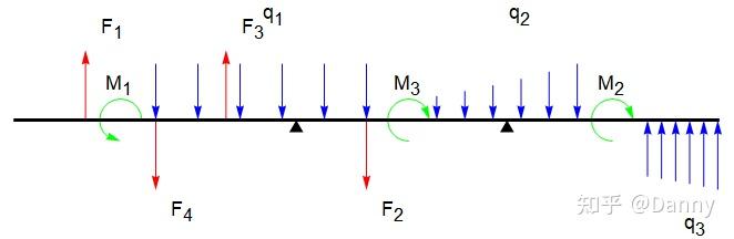
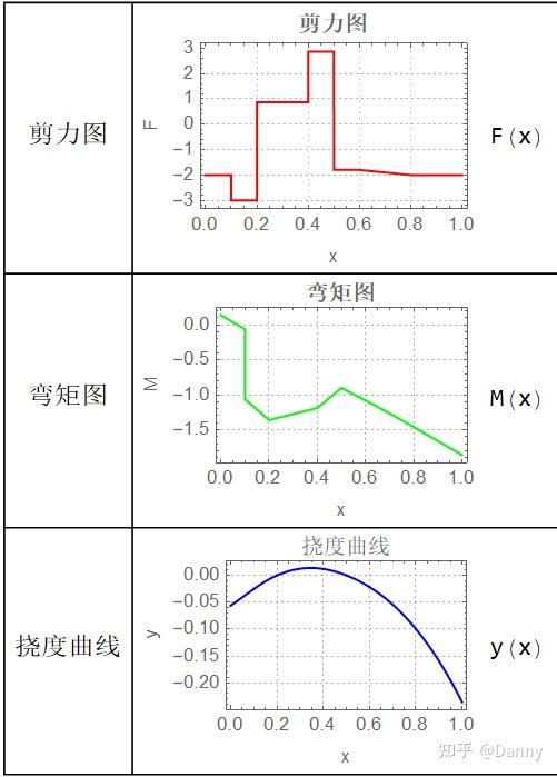
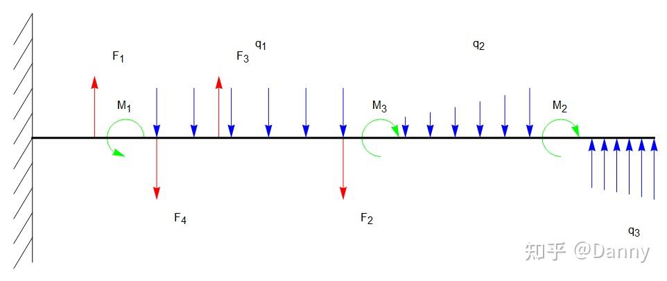
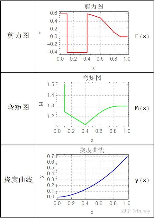
说明一下,剪力图,弯矩图,挠度曲线和受力图没有选用对应的参数,只是作为一个示意。

本文采用CC-BY-SA-3.0协议,转载请注明出处
作者: 得意喵~